


Sensor Tests
The sensor behavior was complex enough that I had to run a number of tests before I was sure I was handling them correctly. This page records the results of the most interesting ones. For these tests, what I’d do is keep an array (or multiple arrays) and each time around loop (or on some other frequency) I’d put the relevant numbers into the next free cell of the array(s). Since there isn’t enough SRAM for the array to be as long as I’d like, I used short arrays and had recording start at some offset from an event, or I’d treat the array as a circular buffer (running off the end looped back to overwriting the beginning, and stop some fixed time after the even of interest. Then I’d print out the numbers in the array(s).
Printed numbers were saved as text, and imported into an Excel spreadsheet for processing and graphing them.
Testing the Algorithm
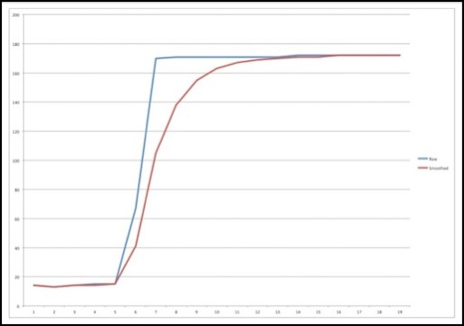
The example I found uses an “alpha” of 1/16, or 0.0625. This takes a long time to adapt to changes in light levels (i.e., it’s doing more “smoothing” than is necessary for what I need). The algorithm can be easily changed to use any 1/N alpha, and I adapted it to use an alpha of 1/2 (0.5 or N=2), which works much better. The following is a graph of samples taken using a test program, showing the raw sensor values (blue), the lightly smoothed (N=2, red)) and heavily smoothed (N=16, green) values:
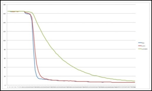
IR Sensor Falling Response Time graphed over 80 cycles of 1.5 msec each
It’s a bit hard to read, but where the raw values dropped from 165 to 10 in 21 read cycles, the fast smoothing did the same drop in the same time (taking only one cycle longer to make the initial drop from 165 to below 65) and the slow smoother took 63 cycles to drop to 10, and 22 just to drop below 65. Each step recorded here took 1,470 micro seconds +/- 10 microseconds (or just under 1.5 milliseconds per cycle).
Looking more closely, you can see how the blue line drops slightly below the red at first, representing how smoothing delays responding to sudden changes (this is probably while the obstacle is still moving in front of the sensor and light is only partially blocked), and then as the sensor value drops steeply, the fast-smoothed curve lags it only slightly, while the slow-smoothed curve lags far behind.
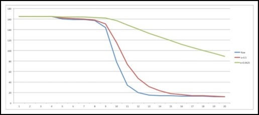
IR Sensor Falling Response Time over 20 cycles
Rising is similar: the raw value actually goes from 0 to 163 (its maximum) in just two steps. The lightly smoothed curve takes 8 steps to maximum and only two to rise above 100, and the heavily smoothed curve takes a whopping 79 steps to maximum, and 15 to exceed 100.
Oddly, during my testing I observed some situations where the fast-smoothing algorithm took more than ten cycles to rise 100 points. I’m not entirely sure what caused that, but there would appear to be some variation in sensor response from one time to the next.
IR Sensor Rising Response Time over 80 cycles
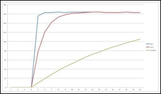
IR Sensor Rising Response Time over 20 cycles
If you’re curious, I generate these graphs by storing each cycle’s current values in an array, the index for which resets back to zero when it gets to the end. When my trigger event (going up by 10 in one cycle) occurs, I print the whole array out to the serial monitor. Then I cut/paste the numbers into a text file, import to Excel as CSV values, and use Excel’s graphing function to draw a picture of a subset of the data points.
Room Light Test
Let’s look at some real sensors and real lighting. For these, I’ve updated my code to use N=4 for the main smoothing (so the red line below is adapting to half the difference after 3 cycles), and I’ve also added a number, called “Adjusted”, that tracks the average over all smoothed sensors with additional N=16 smoothing, which is used to reset the definition of HIGH when ambient lighting changes. This means that if room light jumps by 500 points (a very extreme change), the definition of HIGH won’t change by more that 31 points in a single cycle, and that means that the difference between LOW and HIGH would need to be less than 62 points for a false detection of an occupancy change.
The following chart is from one sensor in a set of four. The sensors are LTR-301 LED phototransistors lit by LTE-302 IR LEDs (set up per my Sensors design), with values recorded for the first sensor in the set. With the IR LED alone illuminated in a room lit with dim LED lighting (no IR component from the room LED lights, sensor readings under 10 with the IR LEDs off) the sensor reported values around 285 for HIGH, and under 10 for LOW, roughly a 140-point detection threshold. With a lamp placed so that it’s exposed 60W bulb was 22” from the sensor, on-axis but up 45 degrees, the sensor reading went up to 450 for HIGH and 50 for LOW, for a 200-point threshold.
Using a program that recorded readings for each cycle (roughly once per millisecond) for a full second, I then placed a solid object blocking the direct light from the bulb (some indirect light still made it to the sensor, and HIGH readings went up to about 340) and recorded the following graph. The X-axis is time in milliseconds, and the Y-axis is the result returned by analogRead, either unprocessed (raw) or after being smoothed.
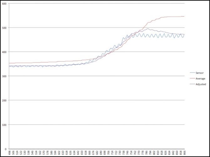
Raw IR sensor (blue), N=4 smoothed (red) and N=16 smoothed (purple) values as sensor goes clear
The above chart shows the raw sensor value (blue wiggly line), the average HIGH value over all sensors (red line), and a line (purple) created from the heavily-smoothed “difference from average” value used in my sensor processing logic added to the average. Note: the reason the blue line is wiggly is that it’s showing the effect of 60Hz AC power on an incandescent lightbulb: the temperature varies over time, although at worst this was about a 16-point swing and the smoothing removed almost all trace of it.
The intent here is that the purple line represents the value actually compared with a smoothed sensor reading each cycle to determine if the sensor is occupied or not. It needs to track room light changes over all sensors, but smooth them out so that the cycle-to-cycle difference between the actual sensor value and the high value is never too large, even on a sudden change.
Now what this shows is interesting. It takes a long time for the light level to rise, and I think that’s mostly in the speed of how quickly I could remove the obstruction (75 msec to full brightness is a long time for a sensor, but a short time for human muscles). This could reflect a variation in room light from someone moving an arm in front of a nearby table-lamp, for example.
As the room light rises, you can see how the purple line initially falls below the blue line, and then about halfway up starts to rise above it. That’s exactly the behavior expected. Additionally, while the maximum cycle-to-cycle variation of the sensor was 10 points, the maximum of the purple line number was just 4.
BTW, I think the reason the red line ends up well above the blue is that some of the detectors are much more sensitive to off-axis light than the one I charted in blue, so the average ended up higher after increasing the off-axis light.
This test showed that my idea of using N=16 smoothing was producing usable results, and gave me an idea of how quickly it would adapt and how closely it would track the N=4 smoothed number I was using for sensor results. Having this as a reference both confirmed that my approach was good, and let me structure the adaptive code that keeps the sensors returning useful results even as room light changes.
Early Testing
My first tests were simply to prove that I could read the sensors accurately and to work out initial bugs in the software. The following records the testing I did at that time.
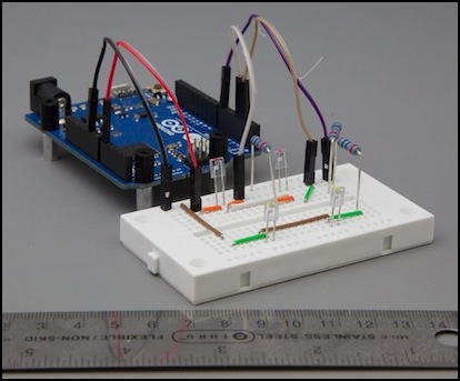
I set these up for initial testing on a simple breadboard (below) which just happens to be wide enough for the track to fit between the two rows. In addition to the four pins on the Arduino, the black wire (top center) connects to the logic ground pin on the Arduino, and the two connectors on the lower left (orange and blue jumpers sticking off the edge) connect to the 12V supply powering the LEDs.
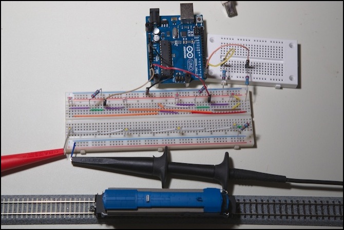
Test rig (this version was using Digital pins 0 and 1, which was a bad idea)
The test rig has LEDs along the bottom (those are the ones with yellow dots on the top, they’re hard to see), with power supplied by two connections on the bottom left. The phototransistors are arranged along the top (the ones with red dots), and these have the wires to the Arduino. The jumpers on the board are a bit of a mess because I had to use ones that would lay flat, since I’m going to put track on top of them, and those only come in specific lengths.
The two things that look like multimeter probes (because they normally are) are connections to my 12V bench power supply, which happens to use the same shielded jacks as a multimeter, so I can use multimeter cables with clip ends to connect to things.
Here’s another picture:
Side View
It may not be obvious, but if you number the sensors from left to right, they’re actually read in the order: 2, 4, 1, 3 or 1, 3, 2, 4 (assuming I vary the digital pin only after reading both analog ones, which is the way my program works). That wasn’t intentional, I just hadn’t thought about how the software would work when I wired them up. The order doesn’t really matter, since it takes about half a millisecond to read all four (at least in the simplest form of my program), and at that speed a train passing in front of them isn’t going to move more than about a tenth of a millimeter between reads, and probably much less.
Test 1
Now my first several attempts didn’t have a running train, I simply wanted to read sensors and print out their values, repeating once a second, so I could get a feel for what the program was doing and how sensitive the sensors were. This used a very simple program that read the four sensors into an array along with the times they were read, printed out the two arrays (time and value) and then paused for a full second before repeating. This let me do some basic testing with ambient light changes (turning lights on and off) and resistor values, to get a feel for how things worked before I spent time on anything more sophisticated.
My initial testing was done with 12K Ohm pull-down resistors, because I misplaced my pack of 10K ohm ones. The LEDs were driven with a 330 ohm resistor, drawing about 30 mA of current off the power supply, so they weren’t as bright as they could be (they’re rated up to 50 mA), but they were at a good level for a long service life and a reasonable light level.
With the LEDs active in a darkened room, all sensors reported values in the 900s (on a 0-1023 scale) in this test. With the LEDs off, they reported values around 300. But with the room lights on, the “off” values climbed to around 700. Part of the problem was that the “room light” was a halogen desk lamp, putting out lots of IR on its own. Unfortunately, that’s also going to be true of any incandescent lamp. There’s enough IR out of a normal bulb, that these sensors are going to report on it. The layout lighting is mostly fluorescent, so it may not be as big of a problem, but I do need to worry about it. A 700-to-900 range isn’t a broad high/low range, and the sensitivity to room light levels was a problem I’d ultimately have to deal with in software.
Test 1b
After another trip to the local electronics store, and returning with a really big pile of resistors (I was determined not to be missing the right size when I needed one, but I still didn’t have a 470 ohm one when I realized I needed safety resistors, so I used 680 ohms for those on the test rig), I swapped out the pull-down resistors for some 2K ohm ones.
I’m tired of running out of resistors in mid-project
This gave much lower values when the LEDs were off, and suitably high ones when on. It’s possible that tuning the 12K Ohm resistors down closer to 8 KOhms would work better, but it looks like “Active Mode” (1-3K Ohm resistors) is going to be of more use for me (further testing confirmed that).
However, it was still very sensitive to room light. With the LEDs turned off, in a dark room with distant incandescent light they read 19, and it’s quite possible that’s coming from me, rather than the lights, since I was sitting in front of the sensors. With a desktop incandescent bulb about three feet (1m) away, behind the light sensors (so it wasn’t shining on the sensitive front part), the sensors read numbers around 70. However, with a desktop halogen light about 18” (0.5m) away, and above them, readings shot up to 300. So these things aren’t very precisely tuned to the 490nm frequency they’re specified for (or else the halogen puts out a lot at that frequency).
With the LEDs activated, and the room darkened, the sensors read about 500. Turning the halogen on at that point made them read 600. So distinguishing the light from the LEDs from ambient room lighting gives me about a 600-to-300 swing (I tested that with a solid object in front of the LED), which is less than I’d like to have, although it could be workable.
Unfortunately the big problem came when I tried to test individual sensors. With light-blocks between each pair, so P1 could only see light from L1, when I blocked P1, the Arduino read a lower value for both P1 and P3 (the two sharing the same output pin, pin numbers #1 and #2 on the test rig). Clearly I did not have a usable multiplexed sensor at this point.
The problem was a stupid error: I had used digital pins 0 and 1, because they were the closest ones. I overlooked the fact that these are “special” digital pins, and you shouldn’t use them if you’re also using USB (as I was), because they’ll give erroneous results due to their connection to the serial controller. Once I move to pins 2 and 3, things worked much better.
Test 2
With the Digital pin problem discovered and fixed, I made my program a bit more sophisticated, so I could test multiple reads. The goal here was to see if doing two reads and discarding the first will improve accuracy. What I found was that the first set of reads after a long delay (tens of seconds) could have the very first read of each sensor bad. But once I started cycling and reading sensors once a second, that went away and the “discard” value was almost always only a point or two (out of 1023) different. I removed the “read twice” code at that point, to speed up the algorithm.
And that broke it. It turns out that there does need to be a delay after the digital pin is turned on to energize the bank. This looks like it could be as short as 50 microseconds, but I found slightly better results with 100 microseconds (and no additional benefit from 200). Now with four sensors in two banks I can read all four sensors in under 700 microseconds.
With that, I started testing different values of R1 and R2, and found 8K+ was too erratic for my use, but values from 2K to 5K worked fairly well, with 5K slightly better than 3K, and 1K significantly worse than 3K. I didn’t test 6K as I didn’t have the right size resistors to easily test that. In theory, the appropriate value will vary based on the sensors in use, from about 2K to about 8K. Later on I reverted to 2K so I was testing a circuit that would work for any normal variation of phototransistor (see test 4).
With bright ambient lighting, “on” was about 750, and “off” was about 500 - 670. With less-bright ambient lighting the difference improved, and in a dimly-lit room with a 50W bulb about 6’ (2m) away behind a lampshade, “off” was 50 or less and “on” was still 600 - 750 (except for my defective sensor, which was now 300 - 500 when “off”). I need to test these under the layout’s fluorescent lighting to see how that works. Although it’s bright, there should be relatively little infrared in that light, so if the detectors really are frequency-specific, that shouldn’t be an issue.
Test 3
The next part was to test my smoothing algorithm. I tried the original example I’d found online, but it took about 30 sensor reads to adapt to large changes, and while that was probably workable, it was much slower than I wanted or needed. This was using an alpha of 1/16, or 0.0625. I decided it would be easy enough to adapt this to an alpha of 1/2 (0.5), so I did.
This didn’t work the first time I tried it (I’d done the math wrong), but after a while if fiddling around and re-checking my math, I fixed it, and found that with alpha = 0.5 even under poor conditions it would adapt in about six cycles (and perhaps less, depending on how far I needed the count to move before considering it to be a state change). With that working, I turned my attention to creating the code that would determine that a sensor was in an OCCUPIED or EMPTY state.
Test 4
With the smoothing algorithm working (and I tested it rather throughly, I thought), I wrote some simple code to keep a couple of recent sensor levels (5 and 10 cycles back) and check against them to look for changes greater than 100 over a multi-cycle period, as the minimum normal variation seemed to be less than 75 and the difference between low and high was never less than about 120 in any of the cases I observed. And I’d noted from my testing that the algorithm would make a >100 transition relatively quickly. After the usual debugging, this worked fine to detect “going low” transitions (when a sensor became occupied), but just couldn’t seem to detect “going high” ones.
I made a number of changes at this point, including switching back to 2K ohm resistors (I’d been using 5K ohm up to now) and creating a second test board I could use at the desk where I do programming, as the electrical bench (i.e., the dining room table) wasn’t really suitable for extensive software debugging efforts, and it was clear I had some kind of software problem.
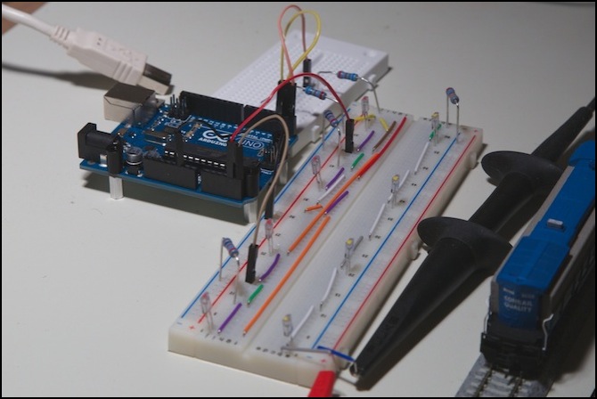
Leonardo with two-sensor test circuit
The second board, using a new set of LEDs and sensors, worked very similarly to the old one. This one was plugged into an Arduino Leonardo, simply to keep me from having to carry the Uno back and forth, and it was built with only two detectors, using the Arduino’s 5V supply to light the LEDs (the extra 30 mA is fine given how little this board is doing). I omitted the safety resistors to keep the small breadboard I was using cleaner. It’s a very simple circuit, and a copy of the one I’d already done, so I was less concerned with accidentally grounding a pin.
The room lighting was slightly different (two indirect 50W-equivalent LED bulbs rather than incandescent/halogen, giving a dimmer light than my electrical bench, suitable for working on a computer), and I was seeing highs around 180 - 200, and lows around 0 - 50 (each sensor was consistent, but one was consistently higher than the other). A “going low” transition occurred over about two or three cycles (and this could have partly been due to the speed my finger was moving when placed in front of the LED; I expect it takes two cycles to fully block the light). A typical reading sequence went: 177, 178, 178, 176, 140, 87 or 210, 211, 211, 200, 136, 68 (I stopped collecting history when the delta exceeded my threshold of 100). This actually made me wonder if my smoothing algorithm might be adapting too quickly, although it seemed to hold things nicely stable over normal variation.
And then I proceeded to dive into the program, to figure out just what was going on, millisecond to millisecond, by capturing a rolling set of samples each cycle for ten cycles, and printing them out for even a slight increase. Note that I don’t print them out each cycle, as that would add tens of milliseconds to the loop, and I want the timing between pin reads to be the real timing.
And there was the problem (or so I thought): the algorithm takes a very long time to rise from 0. In ten cycles, it rose only 13 points on one sensor, and 27 on the other. Here’s the snapshot from the second sensor (starting from zero at cycle 8):
cycle 4319, upwards trap.
0 =168, 1, .
1 =170, 1, .
2 =171, 4, .
3 =172, 8, .
4 =172, 13, .
5 =172, 18, .
6 =172, 23, .
7 =172, 27, .
8 =165, 0, .
9 =166, 1, .
Notice that sensor 0 has also fluctuated by seven points in the same period. I’m pretty sure that’s an artifact of the two of them using the same A/D chip, although it could be from sharing the same analog pin. Either way, that’s part of the “normal variation” I need the smoothing to compensate for and the “large transition” code to ignore; unlike sensor 1 it doesn’t keep on rising too much.
My mistake (or so I thought) was that in testing the smoothing algorithm, I only looked at values every 10 cycles, and saw it reach the final state in only a couple of 10-sample steps, where the high value was a couple-hundred points above the low. What I missed was that during the initial ten cycles, it was on the start of the exponential curve, and not rising much each cycle. After ten steps it was rising about 5 per step, so it only took another 10 or 20 to pass the 100 threshold. At that scale, I couldn’t really see that it fell faster than it rose (in an absolute value sense; as a relative value to the start I expect the rates were similar).
At this point I wrote a short program to capture several hundred cycles, and then print them out, allowing me to graph them (using Excel) on a step-by-step level, to see just what the sensors were doing and how my algorithms were adapting to those changes. I’ve posted those up above. Oddly, what I saw in the graphs were numbers that should have worked to detect a sensor going clear within my 10-cycle window.
Armed with that information, I went back to my main test program (the one with the code to detect high/low transitions that wasn’t working) and added a similar rolling history of the last 200 raw and smoothed sensor readings, and saw this:
Raw (blue) and smoothed (red) sensor readings in main test program
Now that’s what I should see. It’s not quite as pretty as the test program, since the raw values don’t leap all the way up in one step, but it’s still rising fast and the smoothed line is still following it well and also rising fast. But why wasn’t my trigger catching that? The smoothed values take 7 cycles to go from 14 to 138 and after 5 more are at 170. That’s more than enough to trigger my “up by 100 in 5 or 10 cycles” code, so why doesn’t it?
While I was working on that, another puzzle presented itself, I seemed to be seeing a synchronization between readings on two different pins (larger than the one noted above). But with a little checking, I realized that what I was seeing was the effect of off-axis light between my two sensors. There were less than an inch apart (about 2cm), with the LEDs about 1 inch (2.5 cm) from the sensors. When I blocked the light into sensor 0, I was also blocking some of the light from LED 0 into sensor 1. This caused a deflection of about 20 points out of 180 in the value of the sensor. Which indicates how tightly focused the sensor is: I was blocking a bit less than 50% of the light on my test board that could be hitting it, and it was deflecting only a bit more than 10%. I stuck a business card between sensor 0 and sensor 1, and almost all of the synchronization went away. I did still see the other sensor move by a couple of points, which probably represents the effect of higher voltage above the phototransistor when the other phototransistor is off. But this was so minor as to be below the random fluctuations I’m seeing in a dimly-lit room.
And I finally tracked down the mystery of why my sensor wouldn’t detect an upward transition. I had a coding error that prevented my sensor history variables from ever being updated (memo to self: always test for X >= Y, not X == Y when incrementing up to a trigger point, because sometimes X starts out higher than Y). I can’t believe it took me four days to figure that out. Even looking at graphs that proved my snapshot history of the sensor variables wasn’t being compared to the current sensor properly, I never caught on to the basic idea that my snapshot wasn’t being captured at all. Some days I amaze myself, and not in a good way.
