


Model Railroad Wire Ampacity Derivation
Determining the effective capacity (ampacity) of wire used in a model railroad is not a trivial task. And, as I’m not an electrical engineer, it’s easily one I could have done wrong. For that reason I’m providing a detailed description of how I came by the results on my Ampacity page here. If anyone sees anything I’ve overlooked, or done incorrectly, please drop me a note to the address on the About the Site page. Note that there’s a lot of math here. That’s kind of hard to avoid, but I’ve stuck to simple algebra, using formulas derived by others for specific cases. Hopefully I haven’t misused any of them.
And it should go without saying, but I’ll say it anyway: use at your own risk. I’m not an electrical engineer, and I’m not providing professional advice. This derivation is correct within the limits of my knowledge, but those limits may not be as broad as I think they are.
Basic Tables
The tables presently provided are derived from online information. These will ultimately serve as the sanity check on my own tables; if I differ significantly, I’m going to need to determine why.
Normal Wire:
Information in this table came from Wikipedia’s entry for American Wire Gauge (AWG) as well as the Wikipedia Ampacity table. It doesn’t entirely agree with other tables I’ve seen, but that’s one of the problems: every table seems to use slightly different assumptions and ends up with slightly different ratings as a result. In particular, the numbers here are higher than the ones in the magnet wire table down below.
Note that this table assumes copper (Cu) wiring. Additional derating would apply for wires made of aluminum, and pre-tinned wire has slightly less capacity as well.
Magnet Wire:
The magnet wire table is based on a list of standard dimensions for solid-core wire, and ampacity is based on the range of current densities given on the wikipedia page (see magnet wire link above). Skin effect should not be an issue with wires of the size listed here, even at PWM frequencies. Temperature derating is presumably included in these numbers, and I think the “interior” number reflects a worst-case scenario, but I can’t be certain. The numbers appear overly conservative to me.
Adjusting Standard Tables for Model Applications
Actual ampacity for high-frequency (DCC) current in small-gauge low-voltage wire is hard to come by. Ampacity tables (like this one) describe the allowed minimum size of wire for a given current under two conditions: in open air, and in a confined space, given a number of assumptions, one of which is that wire can be allowed to heat to some number up to 90°C. A wire that hot in contact with a typical plastic model should not cause the plastic to deform since polystyrene has a “melting point” of 100°C, but it turns out that that’s not a safe bet, as we’ll see below in the discussion of acceptable heat levels.
Temperature Derating:
Standard ampacity tables typically (but not always) assume an allowed maximum wire temperature of 90°C, multiply the ampacity by 0.82 to get the ampacity at 75°C.
Paired Cable Derating:
If two wires are touching, as in a twisted pair, multiply the ampacity by 0.93. Note that this does not apply if the two wires are separated by more than the diameter of the wire, as they would be in zip cord. It’s interesting that there’s only a 7% derating here, as a back of the envelope guess would suggest each wire has half the ability to shed energy to the environment, and thus should be derated by 50%. Clearly there’s something else at work.
The Hard Stuff
Now for how I did my own tables. I haven’t finished these yet (and the tables aren’t published yet, since I’m still creating them), so the following material may change before I’m done.
Even with a number of assumptions, the math for this isn’t trivial. Conceptually it’s all very straightforward, but finding the equations and constants for various materials, figuring out how to apply them, and putting it together kept me well-occupied for a while. Hopefully I got it right: I haven’t had to do this kind of analysis since college physics.
The basic concept is simple: the useful size of a wire for a given current is limited by two things, the voltage drop in the wire (which gets larger the longer the wire is and increases with the current being carried) and the heating of the wire due to that resistance (which doesn’t depend on length but does depend on the square of the current). For long wires, voltage loss is probably the biggest issue. For short wires, heat may dominate. I’ve reported voltage drops for different lengths and amperages to help identify where this becomes the dominant factor.
In short, the ampacity of a wire depends on:
- Acceptable voltage loss in the wire, which depends on gauge, current, material and length
- The heat produced in the wire, which depends on gauge, current and material
- The ability to remove that heat, which depends on the environmental temperature, as well as how heat is removed:
-- via convection in open air
-- via conduction (or radiation) in a closed space, which additionally depends on the surrounding material
Kinds of Wire
I’m going to look at four use-cases for model railroads:
- Track Bus Wiring
- Track Feeder Wiring
- DCC Decoder Wiring
- Accessory Wiring
The first three make up the train power supply system from command station (or power pack for DC) to the train’s motor. The last applies when dealing with control signals to accessories like switch motors and signals, as well as power wiring to devices such block occupancy detectors or turnout motors that don’t take their power from the track or to LEDs providing light in or on structures. While I’ll look at the train power system in the context of DCC, most of this applies similarly to DC layouts, the only difference being that currents will typically be significantly less (DC block wiring has to support at most a couple of train motors, perhaps ~1Amp, while DCC bus wiring can carry 5 or more Amps).
Environment
One assumption that must be made concerns “room temperature”. While basements are often cool, and assuming 20°C (68°F) would be safe in many cases, that’s not always true. Some model railroads are in garages, lofts or spare rooms. And model railroading happens in summer as well as winter. To provide a safety margin I’m going to use a higher temperature.
Since much modeling uses plastics, the effect of temperature from heated wires on plastic models is of particular concern.
I’m taking a conservative perspective, and assuming a “room temperature” of 30°C (86°F), with a maximum allowed wire temperature of 50°C (122°F), meaning a 20°C rise (more on wire temperature below). I could have relaxed that to 20°C (68°F) room temperature and 75°C (167°F) wire temperature, and probably still have been fine, but there’s some risk at the higher temperature. Wires suspended in air, not touching insulating foam, can safely heat to 75°C (or more, but I’ll use that number).
Room Temperature: 30°C
Wire Heating
As mentioned above, a final assumption is how hot to allow the wire to become in use. The primary objective is to avoid damage to the wire or to models, as this is a more conservative assumption than insulation failure or causing a fire (the other reasons to limit temperature).
For wire in open air, I’m assuming the air can circulate freely past the wire. This may not be the best assumption (particularly if the wire is glued to a ceiling), so treat “free air” as a best-case and realize that a lot of situations may be less than the best. For a wire in a structure (model building or train), I’m assuming the wire is inside a styrene model and its cooling depends on the rate of heat transfer through 2mm of styrene. For wire in or adjacent to a layout (e.g., bus and feeder wires not in open air) I’m assuming the material surrounding the wire is solid styrofoam insulation, as this is more restrictive than wood or having material on only one side would be.
Note that the melting point of copper, 1,084.62°C, is far above the temperatures that become problematic for these other materials. Thus the “fusing point” of copper isn’t an issue here. We’ll have destroyed both model and wire insulation, shorting out the power supply and either shutting the layout down or setting it on fire, long before the wire itself melts.
Most electrical insulation is PVC, which has a melting point of 105°C (221°F). It’s generally recognized that wire temperatures should be kept at least 10°C below this, and often a safety margin of 30°C (a wire temperature of 75°C or 167°F) is used. That’s actually pretty hot, and in most applications we’ll want to aim for a lower temperature.
Plastics are a glass-like structure, meaning that they become “rubbery” above their “transition temperature” (also known as the “glass temperature” and “melting point” although the latter isn’t strictly true) and experience “creep” at lower temperatures. The exact temperature depends on the type of plastic, and what other substances it has been mixed with. Polystyrene tends to be somewhat less adulterated the many other types (which often contain materials to enhance flexibility or other properties), and has a slightly higher acceptable temperature as a result.
Polystyrene plastic has a transition temperature of 100°C in its pure form, but that can range as low as 75°C depending on the formulation and apparently commercial formulations with a transition temperature of 85°C are common. This temperature is the center of a range where the solid material transitions into a rubbery form. Even below it, plastic may become soft enough to deform under its own weight or other normal stresses applied to models (as noted above for PVC). Staying at least 10°C below the transition temperature is probably a good idea. Some other plastics are reputed to have issues above 60°C, but exact information is hard to come by. For plastic that means 75°C might be safe, but 65°C is better. For insulated wire, staying below 95°C should be fine.
For most of the tables, I’m actually going to calculate the results for a 20°C rise over my assumed “room temperature”, meaning 50°C (122°F), to ensure a large safety margin for wires used in or near plastic structures. For wires in control panels or open air, not exposed directly to plastic of styrofoam, I’ll be less conservative and allow temperatures up to 75°C.
For voltage loss only the wire temperature matters, and it’s at most a one-gauge improvement from 50°C to 75°C, so for bus wires (the ones most affected by voltage loss, and also the ones most likely to be in open air) the result of allowing that higher temperature do not substantially alter the ampacity, but there is an improvement so I’ll calculate those tables allowing for it.
Wire Max Temperature: 50°C in structures, 75°C in open air
Acceptable Voltage Loss
This is a core assumption, and somewhat arbitrary. How much voltage are we willing to lose in a wire? The answer depends on what we’re doing with it. For normal household wiring, often a number of 3% to 5% is used, but this is only part of an end-to-end transmission system. And in any case, we’re dealing with low-voltage model trains, not lamps.
Let’s assume N-scale DCC as the most severe case (someone working with a garden railway at much higher voltages might draw different conclusions). A DCC power station (command station or booster) puts out a nominal 12V (DCC RMS) signal. A decoder must respond to at least a 7V signal. That means we could lose 5V (or 42%) of the source and still work, but clearly that’s not a very desirable state. DCC decoders pass through a fixed percentage of track voltage to the motor for a given throttle setting, which defines the speed. It’s probably desirable for track voltage to be relatively consistent across a layout. There is also going to be voltage loss in the track, in the on-train current pickups, in various connectors, as well as in the bus wire, track feeders, and decoder wiring.
Voltage loss in the track feeder is limited due to the relatively short length, likely under a foot, but perhaps more if you include wiring to occupancy detectors and circuit breakers between the bus and the track. The lower currents typical in feeders (which support at most a couple of train motors each) is also a factor. Even at four feet, loss is going to be under a tenth of a volt with the wire gauges normally used. This can rise to around 0.2V for larger or multiple motors totaling an Amp or so on typical wire (e.g., Kato’s 24ga feeders). So I’m going to budget 2% as the normally acceptable voltage loss in feeder wires (that’s 0.24V). Track and related connectors can be assumed to lose several additional percent (hopefully not more), and completely arbitrarily I’ll assume that’s another 3% (0.36V).
So, from the above I’m losing 5% (0.6V) in track and feeders. Let’s assume loss in the decoder wiring is negligible (I think it is), then if I were willing to lose 20% (2.4V, taking track voltage down to 9.6V) my buss loss budget would be 15% (1.8V). Let’s assume that’s the worst case upper bound on loss. What this means is that track voltage, and thus train speed, can vary by 15% from one part of the layout to another. That seems a bit high to me, but not fundamentally broken. However actually using this margin isn’t recommended.
In the interest of consistent behavior I’m going to set a lower target for “normal maximum” loss of half that (10% overall, meaning 5% in the bus). Thus, voltage at the decoder would vary from 10.8V at the “consistency” target down to 9.6V using the worst-case loss. Even the worst is comfortably above the 7V minimum. And keep in mind this is defining a worst case, and real-world voltage loss isn’t likely to be that high. I’ll also allow feeder loss to be slightly higher in the worst case and assume a small loss in decoder wires. That actually puts me closer to 25% total loss in the worst case, taking voltage at the motor down to 9V. I wouldn’t want to run trains that way, but I have no doubt they’d work unless there was something seriously wrong in the track. My preferred “worst” number works out to 11% total loss, meaning 10.7V at the motor.
Accessories are probably somewhat variable in their needs. Lets assume we want voltage to be no less than 10V from a 12V supply, that’s about a 16% loss. Allowing for some loss in connectors, I’ll use 10% (1.2V) as a maximum upper bound on acceptable accessory wiring loss.
Thus, acceptable losses:
- Track Bus: 5% normal or 15% worst-case
- Feeders: 2% normal (a worst-case value of 5% is used for the table colors)
- Decoder wires: ~0% (meaning less than 1%, a worst case of 2% is used for table colors)
- Accessory wires: 10%, 15% worst-case
More Assumptions
Finally, I need to account for the insulation used on the wire (insulation keeps in heat, not just electricity, so it makes the wire hotter). And different kinds of insulation conduct heat differently, and come in different thicknesses. I’m going to assume PVC insulation (except for magnet wire, where I’m assuming one of the usual compounds used for that). I’ve collected a lot of data on typical PVC and magnet wire insulation thicknesses, and will use that for their respective types of wire. For commercial AC wire, which is typically insulated with PVC in a nylon coating, I’ve accounted for the nylon as well although it has little actual effect.
Dimensions
When dealing with real-world objects like wire, sometimes the source material isn’t using the same set of dimensions that I want to use. Metric measurements can be in meters, kilograms and seconds (MKS) or centimeters, grams, and seconds (CGS). I’m using MKS for all of my calculations. Converting between the two is easy, but important to remember to do. Wires additionally usually use dimensions in millimeters, which need to be converted to meters or square meters for use. Again easy to do, but for space reasons I’m using the millimeter and square millimeter numbers in the tables, even though my math is in MKS, so there are conversions back and forth I need to remember to do. Thankfully I’m using Excel for this, so once I get the formula right, it’s easy to apply it to a whole table’s worth of sizes.
U.S. units use the English system (feet, pounds and seconds). Further, wire is described in “mils”, which are thousandths of an inch (one mil = 0.0254mm). And wire cross-section is in “circular mils”, which is a very odd unit referring to the cross-sectional area of a wire with a diameter of one mil (and NOT a wire with one square mil of cross-sectional surface). A circular mil is 0.000506707479 mm2.
Wire dimensions in American Wire Gauge (AWG) have equivalent dimensions in mils or millimeters, but these vary slightly from one manufacturer to another. There’s actually something of a standard behind this (although apparently not always followed exactly). I’m computing my wire dimensions based on typical stranded wires, using the “standard” thickness for the individual strands. Real wire may vary somewhat from these numbers, but it’s unlikely to have a major effect on capacity. I’ve also used data for some common metric wire sizes where I could find it. There are other wire sizes in use (and other standards, such as British Wire Gauge) than those I have listed.
Heating and Cooling
Wires carrying a current lose some power due to the resistance of the wire. That lost power is converted to heat, which raises the temperature of the wire. If a wire kept all the heat it produced, it would get hotter and hotter until it melted. But a hot wire in a cooler environment will lose heat to the environment, and the hotter it gets, the faster it loses heat. A heated object will reach an equilibrium at the point where heat is being lost at the same speed it’s being gained. Heat transfer is calculated in Watts per area (the area being the surface of the hot object). Since the surface area varies linearly with the length, and heat production does too (because resistance increases with length), once we figure this out for a given length, like one meter, it’s true regardless of the length of the wire.
So what we need to do is determine the rate of heat loss at the highest temperature we want the wire to be (which will vary as described above based on some assumed environmental factors), and then work backwards from that number of Watts being exchanged to the environment at that temperature (which additionally depends on the environment), and from that to the number of Amps required to produce that many Watts. That, then, is one limit on the ampacity of the wire: the current that produces the maximum acceptable level of heat in a wire at thermal equilibrium with its environment. There are a couple of complications to that.
First, a wire in air cools at a different rate than a wire surrounded by some other object. For our environments, the maximum acceptable current (i.e., the degree of cooling) will be highest in air, and lowest inside the solid materials used in a model railroad layout (which tend to be good insulators, like wood or plastic), so ampacity in a constrained environment will define our “worst” maximum current.
Second, a wire cools at a rate that depends on the difference between its temperature and the environment’s temperature, so we have to make an assumption about what “room temperature” will be, as described up above. If you model in a much hotter environment (like the Australian outback, or mid-summer Florida) your wire can carry less current. Finally, a wire in air cools at a different rate depending on its angle (air moves up when heated, so a vertical wire doesn’t cool as well as a horizontal one). Most wires in air on a model railroad will be horizontal, so we can probably simplify to the horizontal case as our “best” value.
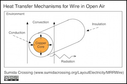
There are three mechanisms that transfer heat from a hot wire to the surrounding environment: conduction, convection and radiation. These all come into play for an insulated wire in open air. Because copper is an excellent conductor of heat, we can assume that heat is available at the surface of the wire for removal at the rate that heat is produced within the wire, as all other transfer mechanisms will be slower that that of conduction through the copper wire to reach the surface (see below for the numbers to back that statement up).
Heat must conduct through the insulation on the wire, and then from the surface of that it will transfer by both radiation and convection. The latter depends on air moving past the wire, and will not apply if the wire is adjacent to some other object. A wire against a solid on one surface may still transfer heat by radiation in other directions, but will transfer via conduction to the surface. As this is an intermediate case between open air and being embedded within a solid, it won’t be considered further here.
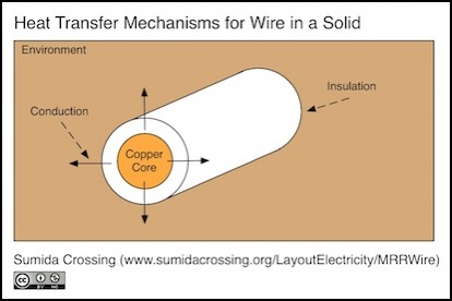
A wire embedded in another substance can only transfer heat by conduction from the insulation to that substance.
Cooling of a surface in air is by convection, where the air adjacent to the surface of the wire is heated causing a density change, the hotter (less dense) air rises, sucking in cooler (denser) air to contact the wire, and the process repeats. With the right set of conditions this creates a “laminar flow” of air past the wire, and a constant exchange of heat to “room temperature” air. In a closed space, things get more complicated as the “room temperature” will increase over time, unless it too can exchange heat somehow. I’ll cover this issue more in the discussion of the application of the ampacity tables to various situations.
In free air, some heat is still transferred by conduction. The ratio is reported to be ~4.36:1 (convection:conduction), or about 81% by convection. Still, there’s enough that the conductive rate of transfer to air needs to be considered as well. A bit of reading suggests that it shouldn’t be that high, unless the wire is corroded, as emissivity of bare polished copper is quite low. Also, as we’re dealing with insulated wire, conduction will be the mechanism of transfer through the insulation. And in wires embedded in some other substance, conduction to that substance will likely be the limiting factor. There could also be also conduction along the wire if the ends of the wire connect to something cooler than the wire itself; with a long enough wire that can be ignored. In a short wire connected to circuitry, the circuitry may be hotter than the wire, and heat added via conduction though the wire.
Resistance
Heat is produced in a wire fairly simply: when volts are lost in the wire due to resistance the “lost” power becomes heat. For DC currents this is calculated quite simply, using our old friend Ohm’s Law: V=IR, for voltage in volts (V), current (I) in amps, and resistance (R) in ohms. The energy turns to heat and raises the temperature of the wire. This is called Joule heating, and the heat is measured in Joules, or more usefully Joules per second. A Watt is one Joule per second, and that’s commonly used as the unit for heat production and transfer, which makes it easy to relate the heat to the power loss in the wire. The amount of heat produced is described by a version of Joule’s Law, P = I2R, where P is in Watts (and I and R are as above). Note that resistance in a wire depends on the length of the wire. While this is usually given in ohms per kilometer, this will be normalized to ohms per meter for use in these equations. In the end, we’ll balance heat produced per meter against heat transferred per meter, and the lengths will cancel out (and thus the length of the wire won’t matter).
Resistance in a wire isn’t a constant. It’s derived from the composition of the wire (e.g., copper, but even that can vary from one wire to another by several percent). It decreases with increased cross-sectional area of the wire (meaning based on thickness, or wire gauge: bigger wires have less resistance). And it increases with temperature (hotter wires have more resistance), so we need to factor in how high resistance will be at the maximum temperature of the wire, as that’s the worst case situation. Fortunately there’s a simple relationship for that.
The DC resistance (Rdc) of a length of wire depends on a number called the “resistivity”, multiplied by the length and divided by the cross-sectional area (Rdc = (ρL)/A, where ρ is resistivity; this is a form of Pouillet’s Law). Resistivity for copper can vary with the type of copper, and is higher for tin-plated copper, but the numbers are well documented for wires at a temperature of 20°C (68°F). The resistivity of soft annealed copper (the typical material for the wire in question) at 20°C is approximately 1.72 x 10⁻⁸, which comes from the International Annealed Copper Standard (IACS). I’ve also seen 1.673x10⁻⁸ used, but this appears to be for some other form of copper. The number for tinned copper is not well documented, but working backwards from some published resistances for one brand of tinned copper hook-up wire gave me a number of about 1.88 x10⁻⁸.
Correcting for temperature is simply a matter of multiplying the difference in temperature from 20°C times a constant (called the temperature coefficient, 0.00393 for annealed copper), adding one, and multiplying times the resistance at 20°C. This is barely a 4% increase at 30°C, but it’s a 12% increase at 50°C and a 31% increase at 100°C, so it needs to be accounted for when working with higher temperatures, and I’ll include it for all.
Skin Effect and Resistance
There is another factor that can apply when AC current, such as DCC, is involved: the “skin effect”. This occurs in wire carrying an AC current, and reflects the tendency for the charge to move to the outside of the wire due to “eddy currents” in the wire. The higher the frequency, the less of the actual wire is carrying the current, and the higher the resistance. Remember the resistivity bit above: conduction depends on the cross-sectional area; if you divide by a smaller area, you get more resistance, which is why thin wires carry less current than thick and why wires that aren’t using their centers carry less than ones that are.
An exact solution for the impact of skin effect on resistance is rather hard, and most formulas representing such solutions are for the special case of 60Hz or for MHz frequencies, and the latter are described as not being applicable to “low” frequencies. So I’ve used an approximation rather than an exact solution.
The current-carrying capacity of the wire’s material effectively decreases logarithmicly as you move away from the surface towards the center, meaning resistance increases in the same manner. The skin depth is the depth within the wire at which current-carrying ability is reduced to 37% of nominal (1/e to be precise). So a wire of twice that has an effective resistance slightly higher than it would for a DC current, although the effect is relatively minor. As the wire’s radius grows larger than the skin depth, the effect become increasingly important.
A rule of thumb (see this series of blog posts) is that for wires of radius less than the skin depth, the DC resistance can be used (it might not be exact, but it’s within a couple of percent) and for larger wires it can be approximated as if all of the current were flowing uniformly in the part of the wire down to the skin depth. As we’ll see below, at DCC frequencies the skin depth is about the radius of a 16ga wire, so wires of 16ga and smaller can ignore skin depth for DCC.
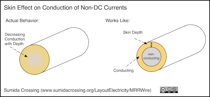
So, assuming we know the skin depth, we can calculate the area of the inner cylinder defined by the total radius minus the skin depth (Ai=(rw-s)2, where rw is the radius of the wire and s is the skin depth) and then subtract that from the total wire’s area (Aw=(rw)2) to get the area used for conduction (i.e., Ac = Aw - Ai). From that, the AC resistance of the wire can be calculated.
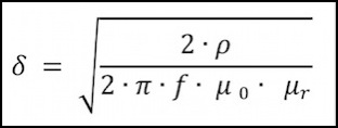
There’s a formula (per wikipedia) for computing the skin depth from the frequency of the alternating current, which is:
Where:
δ = skin depth (in meters, which I convert to mm for comparison to wire size)
ρ = resistivity of the conductor in ohm-meters (1.7241x10⁻⁸ for copper)
f = frequency (Hz)
μ0 = absolute magnetic permeability in Henrys/m (1.2566370614x10⁻⁶ )
μr = relative permeability of copper (0.999993585)
Note: as described here, and shown in the formula above, the formula can be stated in terms of the absolute magnetic permeability of copper (μcu), or in terms of absolute magnetic permeability (in vacuum) times copper’s relative permeability (μ0 x μr ). The latter is more common, as copper’s absolute permeability isn’t always given in texts. But the two formulas are saying the same thing, and either can be used.
Also, as noted above I’ve seen resistivity defined as 1.673x10⁻⁸ (which I think is for non-annealed copper) instead of 1.7241x10⁻⁸, but most wires use annealed copper, and the number I’m using comes from the International Annealed Copper Standard (IACS).
DCC is a variable frequency signal, so the actual skin depth changes from instant to instant. Calculating for the peak DCC frequency (10,204 Hz, assuming worst-case variation in signal), which gives us the shallowest depth, δ is 0.66 mm. Calculating for the more typical 8kHz DCC frequency it’s 0.74 mm. In a long DCC track bus using heavy-gauge wire there will be some impact on resistance, and hence voltage loss in the bus wire, from skin effect. This is worth including in determining ampacity for bus wires, since voltage loss will be the primary limiting factor in long wires.
As per the rule of thumb above, skin depth at DCC frequencies is about the same as the radius of a 16ga wire (0.64mm) thus wires of that size are lower can effectively have skin effect ignored at DCC frequencies. Some simple math for larger wires shows essentially no change at 14ga, a 7% increase in resistance at 12ga, and a 20% increase in resistance at 10ga. However the improvement (reduction) in resistance going from 12ga to 10ga is about three times the amount lost due to skin effect, so there’s still a substantial net improvement in current-carrying capacity for the larger wire, even with DCC in use. In the worst possible case of 10 Amps over a full-length (15 foot or 5m) bus, the extra voltage lost to the skin effect is around a tenth of a volt, or around 1% of the total voltage. This is low enough that the skin effect can be ignored. In short: if you need heavy wire, use it, even for DCC.
Proximity Effect and Resistance
Related to Skin Effect is something called Proximity Effect that comes into play when two (or more) wires are closely parallel, as can happen in a DCC bus if you twist the wires. Data on this has been hard to find (most information is about wires with different utility AC phases, rather than wires with phases that are inverted relative to each other as is the case in a pair of wires forming a DCC circuit). Some sources suggest that for two wires, this has negligible effect. However that statement was likely made in the context of 50Hz or 60Hz utility power, not 8kHz DCC signals. This is something I need to find out more about.
The effect of skin and proximity effects on effective resistance to an AC current is nicely summarized in this PDF.
Radiation
No, not the kind that results in flesh-eating zombies. Radiation is a method of heat transfer, but not a substantial one for solids that are not hot enough to glow. Radiative cooling follows the Stefan-Boltzmann Law and depends on the absolute temperature of the conductor and its coefficient of emissivity, which is a measure of the ability of the surface to radiate heat relative to a “black body”. Coefficients close to 1 are good radiators, coefficients close to zero are not. Polished copper has a coefficient of less than 0.05. Plated copper of about 0.02. Plastics, however, have a coefficient around 0.91 which may affect cooling of jacketed wire by radiation.
The SB law for power radiated by the surface of a cylinder is:
source: wikipedia
where:
P = power (watts)
2𝜋rL = surface of a cylinder of radius r and length L (in m2)
ε = emissivity coefficient of surface
T = thermodynamic temperature (temperature in Kelvins, 293.15K for 20°C, 303.15K for 30°C).
A bit of simple math shows that for bare wire, emission ranges from 9 W per meter of wire for 10ga wire @ 100°C, to less than half that at 30°C, but with insulation this drops to less than half a watt at 100°C and a quarter-watt at 30°C. The numbers drop rapidly for smaller wires, and at 20ga are about 1/3 the value of 10ga.
Since most of the wire in question is insulated, there’s going to be some benefit. For a bare 30ga wire at a low temperature, about 22mW/m can be radiated, and for plastic-jacketed wire this rises to 393mW/m. This is considerably above the power loss in small wire (3mW/m in 30ga @ 100mA), which suggests that radiative cooling of insulation is worth considering. Total heat flow may still be limited by conduction from the wire to the insulation or by environmental factors.
Conduction
Conduction is the principle method of heat transfer between solids. For a cylinder wrapped in a jacket of material (e.g. insulation), the conduction through the jacket is defined by:
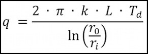
source: Fund. of Momentum, Heat and Mass Transfer Fifth Ed., Welty et al, pg. 206, example 1.
where:
q = heat transfer (in W/m)
k = thermal conductivity of the jacket material (in W/m °C)
L = length of the cylinder (in m)
Td = difference between inner and outer temperatures
ro = outer radius (in m)
ri = inner radius (in m)
Note: for two wires in contact carrying the same current, multiply by 0.5. This is conservative, but will do for now (as noted at the top of the page, this probably isn’t a good assumption and I need to come up with a better one).
Some typical thermal conductivities (from insulators to conductors):
air: 0.024
insulation foam (XPS): 0.034
polystyrene: 0.14 (some sources have lower numbers, likely reflecting EPS/XPS)
hardwood: 0.15 (likely also applies to plywood)
PVC: 0.19
copper: 401
Note: 0.380 for non-pure sample at ~50C per Natick Labs doc (0.372 @ 20°C, 0.389 @ ~75°C), but these are in milli-Cal/cm-sec (need to convert).
Note that air is a really good insulator, which is why convection is more important for it than conduction.
Conduction through PVC insulation of ordinary thickness ends up being around 17 to 72 Watts/meter @ 50°C. Since PVC has the largest value in the list of conductivities above, it won’t be a limiting factor in conduction (i.e., if the wire is buried in wood, wood will conduct less heat even in a thin layer, and thicker layers conduct less). Thus this establishes an upper bound on conductive heat loss unless we embed the wire in aluminum or some other conductor. As we’ve already seen that radiation heat transfer is at least an order of magnitude lower, that could be the limiting factor. However, we still have to look at convection.
Convection
Convection is the principle method of heat transfer from a solid to a “fluid”, which includes a free-flowing gas. And it’s hard to calculate.
One core formula for convection is Newton’s Law of Cooling, q = hc x A x dT, where q is the heat transferred in Watts, hc is the convective heat transfer coefficient (in W/m2°C), A is the surface area (in m2), and dT is the difference in temperature (from wire to air in this case). While hc for air ranges from 5 to 50, the specific value to use depends on the medium (air) and the situation (a horizontal cylinder will be the assumption here; the values would differ for vertical wires somewhat, but wires in open air on a model railroad are typically horizontal). Calculating hc turns out to be hard, and the formula on wikipedia is only valid for large diameter cylinders (like pipes).
References
In addition to the sources cited in-line, the following were used:
THERMAL CONDUCTIVITY OF POLYSTYRENE: SELECTED VALUES, Technical Report 66-27-PR, by Carwile, Lois C. K. and Hoge, Harold J., U.S. Army Natick Laboratories
Wikipedia, List of Thermal Conductivities
Thermal Conductivity of Some Common Materials and Gasses, The Engineering Toolbox (www.engineeringtoolbox.com)
