


Sensor Smoothing
When working with analog inputs, sometimes one value read in a series will be significantly different from the preceding and following ones. This can be due to a number of factors, but usually these factors aren’t important (e.g., electrical noise, a collision sensor detecting vibration in itself, etc). The solution to this is called “smoothing”, a method for adapting to longer-term changes while limiting the impact of short term ones. These are usually based on some form of moving average.
There are a vast number of smoothing algorithms, and some sensor controllers implement these in hardware so you don’t have to program them in software. But sometimes it’s useful to have a simple one that you can apply in software, and I’ll describe the behavior of a set of algorithms based on “exponential weighted averaging” where the exponent is a reciprocal of a power of two. Using a power of two as the exponent allows for more efficient execution of this smoothing in a simple processor like the Arduino.
This is based on an algorithm described by Alan Burlison on his website, which avoids floating point math and division operations, both operations that take “forever” on a chip this simple, given the speeds I’ll be working at.
Digital Filters
Specifically, the solution to a couple of my problems is a technique, or rather a set of techniques, called Digital Filtering. To even out the fluctuations in the sensor reading due to noise in the wires, people walking past the light, and similar things, a digital “low pass” filter is used. To detect large-scale changes when a tram blocks the light from the LED, and separate those from random variation of the sensor readings over time, a digital “high pass” filter is used. Both of these are software algorithms I can write (or rather copy and modify from people who have done similar things before).
Many people who set out to create low-pass filters don’t do this very efficiently. I’ve seen programs that stored past values and recomputed an average each time. That’s a lot of extra instructions for something you want to do often (it’s fine if you’re checking a sensor once a second, but not if you’re checking a half-dozen once a millisecond). Using an Exponential Moving Average only requires the current sensor reading and the last computed average to implement a low-pass filter. Done efficiently, this is very fast.
The basic idea of an Exponential Weighted Moving Average (see “Exponential Moving Average” in the wikipedia Moving Average link above) is that each new sample is multiplied by a “weight” between zero and one, and the past average is multipled by one minus the weight, and the two added to form a new average. The closer the weight is to one, the more important recent samples are, and the more quickly the average will adapt. Conversely, the closer the weight is to zero, the slower the average will adapt.
With reciprocal powers of two (e.g., 1/2, 1/4/ 1/8, etc), the fastest-adapting one is 1/2, and higher powers of two take increasingly long times to adapt.
The Algorithm
The “time” to adapt depends on the frequency of samples collected and averaged. If you collect samples once a millisecond, an algorithm that converges in 10 steps takes ten milliseconds to converge, while if you collect samples every 20 milliseconds, the same algorithm takes 200 milliseconds (two tenths of a second) to converge. Choosing the right algorithm thus depends both on how often you are collecting and averaging new data readings, and how quickly you need to be able to respond to changes.
The actual calculation is quite simple:
newval = (alpha x sample) + (1 - alpha) x oldval
or to put it a bit closer to what we’re going to be doing, for power of two N (where N= 2, 4, 8, etc):
value[i+1] = ( (1/N) * sample) + (1 - (1/N) * value[ i ])
Alan’s version of the algorithm makes some clever adaptions based on the fact that N is a power of two to perform this math in a fixed-point representation using bit-shifting to avoid division (Arduino processors can’t do division). His original implementation was for sensors scaled to a 0-100 range, which allowed him to work with ints (if you can do that, working with ints is better than what I’m doing). But analogRead returns 0 - 1023, and to work with that, the intermediate value needs to be kept in a long rather than an int.
Using alpha=1/2 yields an extra optimization, as one of the multiplies can be removed. It also uses fewer shifts (each bit shifted is one instruction cycle), so it’s faster there too. In general, the larger N gets, the slower the smoothing will be (although for most purposes it’s way too fast for the differences between the various values of N to matter in most applications).
Since I want to work on a number of sensors at once, I’m keeping them in an array of sensors, and breaking value[i] and value[i+1] into separate arrays, so I originally had three arrays the size of my number of sensors: sensorValues (the newly read readings), interimValues (my fixed-point moving average in a long), and smoothValues (my sensor readings after smoothing). Eventually I realized that all I needed to save was the “interim” value, which is the moving average in fixed-point form. When I need to use it as a normal int I can convert one value back to an int (the second line that generates “smoothNxxValues[i]”) where it’s needed.
I’ll leave the longer version here for reference, see the library for the new version.
int sensorValues[SENSORS];
int smoothValues[SENSORS];
long interimValues[SENSORS];
// alpha = 1/16, with fixed point offset of five bits (multiply by 32)
// multiply by 32 divide by 16 is multiply by 2 (left shift 1),
// while multiply by 15/16 is multiply by 15, then right shift 4
// max val is 1024 x 32 x 15 = 491,520 so interim must be long
interimN16Values[i] = (long(sensorValues[i]) << 1) + ((interimN16Values[i] * 15L) >> 4);
smoothN16Values[i] = int((interimN16Values[i] + 16L) >> 5);
// alpha = 1/2, with fixed point offset of five bits (multiply by 32)
// multiply by 32 divide by 2 is multiply by 16 (left shift 4),
// while multiply by 1/2 is right shift 1 (eliminates an extra multiply operation)
// max val is 1024 x 32 x 3 = 98,304 so interim must be long
interimN2Values[i] = (long(sensorValues[i]) << 4) + (interimN2Values[i] >> 1);
smoothN2Values[i] = int((interimN2Values[i] + 16L) >> 5);
Note that interimN2Values and interimN16Values are the smoothed values in fixed-point form. As mentioned above, you don’t actually need to keep both these and the “smoothed” equivalents around. Because of the rounding used to generate the int versions of the smoother versions, it’s best to store the long interim values and just generate the smoothed ones on the fly as needed.
Adaption Rates
I wrote a simple program to execute several algorithms against “before” and “after” values, so I could chart them. In all of these, at time=0 the sensor is returning the “before” value, and at time =1 and later, the sensor is returning the “after” value, so the chart is showing how long (in read-and-smooth cycles) it takes each algorithm to adapt to the new value. In the diagram below I’ve charted the rise from a sensor reading of 10 to one of 300 over 50 cycles, for N = 1/2 (blue), 1/4 (red), 1/8 (green) and 1/16 (purple).
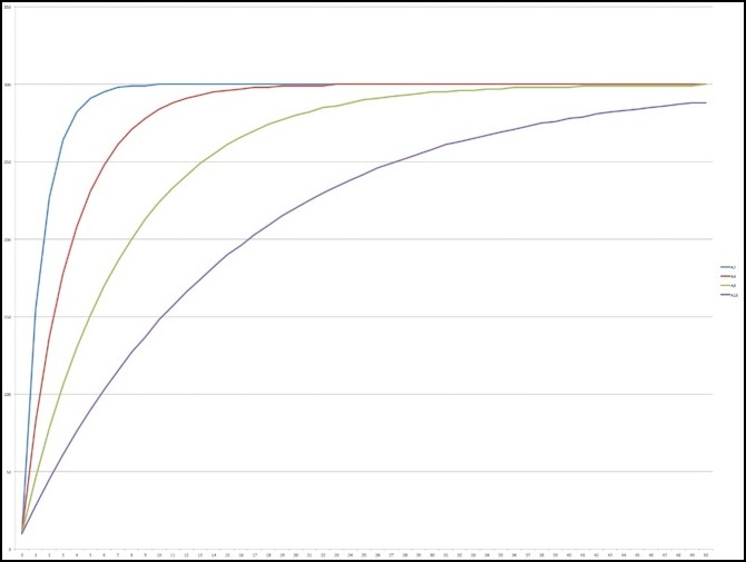
Adaption from 10 to 300 over 50 cycles for A=1/2, 1/4/ 1/8 and 1/16
What’s worth mentioning here is that for a new value of 300, at step 1 the average value is very close to 300/N (so 150, 75, 38, and 19 respectively). The actual values were (155, 82, 46 and 28). Counting “converged” as meaning “within 1% of the final value”, N=2 (alpha = 1/2) took 7 steps to converge, N=4 took 16, N=8 took 34 and N=16 took 70 (even after 100 steps, N=16 hadn’t quite reached 300; it was 299 from step 84 onwards). A more useful measure might be how long it takes to get halfway. For N=2 that was step 1 (pretty much by definition), while for N=4 is was step 3, for N=8 step, 6 and for N=16, step 11.
Let’s consider a smaller change: going from 100 to 150. The curves look similar so I won’t bother with the graph. To get halfway (125) for the four algorithms took 1, 3, 6 and 11 steps. Seeing a pattern? Looking at 10 to 1010 yields 2, 3, 6, and 11. The only reason N=2 was different was a bit of rounding error: at step 1 it was 505, halfway from 0 to the high value, but the starting value was 10, so halfway to the end value would be 510 and it wasn’t quite there.
Let’s look at decay curves. Here’s the graph for 150 down to 100: it looks pretty much the same as the rising curve.
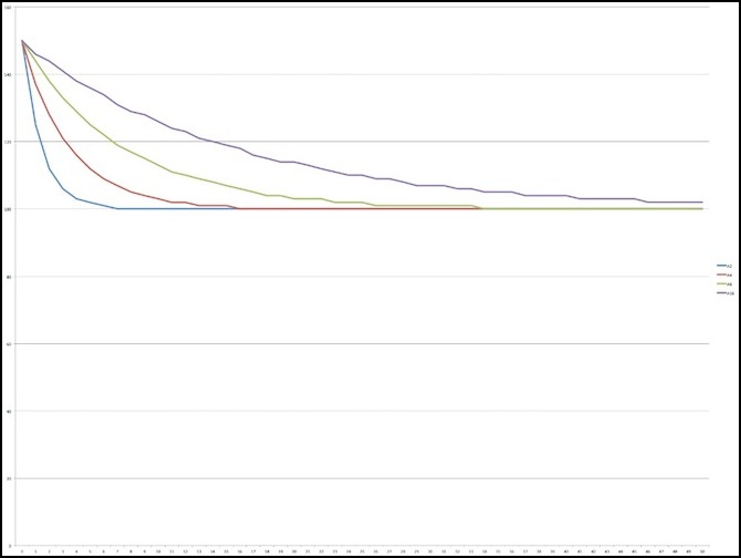
Adaption from 150 to 100 over 50 cycles for A=1/2, 1/4, 1/8 and 1/16
In terms of metrics it’s the same too: from 150 to halfway (125) took 1, 3, 6, and 11 steps again.
What this means is that the absolute rate of change varies depending on how big the change was, so if you’re looking for a 10-point change, it makes a big difference if the actual value jumped by 20 points or 200.
Smoothing Speed
The other difference between the algorithms besides how quickly they converge on a new value is how much processing time they take. Frankly, compared to the hundreds of microseconds it takes to read a value from a sensor, the difference between them is negligible.
Taking the four algorithms described here, packaging them as a function call that processed a set of 8 sensors (so the function call overhead gets spread over the eight of them) and then calling that 1,000 times (and subtracting some other measured overhead) gave me timings for a single sensor smooth of N=2: 7.17 microseconds (usec), N=4: 8.06 usec, N=8: 9.12 usec, and N=16: 9.38 usec.
So regardless of which is used, the variation between them is barely two and a quarter microseconds per sensor read. Even knowing I’ll be doing between 4,000 and 8,000 of these per second in my application, that a total difference of less than 18 milliseconds per second (or 1.8%).
A more useful number is how much delay this adds to a cycle around loop(). In my application, I’m probably going to take about 2 milliseconds to make one loop, and I’ll be processing at most 8 sensors. This means that the longest algorithm adds 75.04 microseconds per 2,000, or 3.752%. The shortest adds 57.36 usec, or 2.868%, so there’s just over a 1% variation in the effect on the application timing. This tells me that I can use any of these algorithms without needing to worry about this aspect, even for the fairly time-sensitive application I’m planning.
Using With IR Sensors
Now the reason I’m concerned with this is that I want to process the sensor readings coming from a bunch of Infra-Red Phototransistors that I’m using to detect moving trains. The values reported by these jump around quite a bit, due to environmental noise and random room lighting changes (unfortunately a lot of room light has an infrared component). In a dimly-lit room, “off” is very close to zero (below 10), while “on” varies from around 250 to 500 the way I have them set up, depending on the particular LED and sensor. (there’s a lot of individual component variation).
So what this means is that if I want to detect an upward move of 100 points, and I’m sampling my sensor every two milliseconds, N=2 will do this in 2 msec (1 cycle), N=4 in 4 msec (2 cycles), N=8 in 8 msec (4 cycles) and N=16 in 14 msec (7 cycles).
For an N-scale model train, 40 kph (24 mph) is about 74 mm/sec, or 0.074 mm/msec. So even with N=16 the train will barely move one millimeter before I detect it, assuming I’m measuring an offset of 100 out of 300 as detection.
If I want to use the halfway mark, ((300 - 10)/2) + 10= 155, then this becomes 1 step, 3 steps, 6 steps and 11 steps as described above, but even then, when using N=16 the train is still only moving 1.63 mm before it is detected.
So any of these algorithms will work fairly well. Higher values of N will ignore noise better. But even N=2 is going to ignore a single sample that’s less than twice my detection threshold. So if I’m looking for half the difference in sensor levels (150 in a dim room), then a random event would need to be 300 / 1024 (or about 1.5 volts) to cause a false positive. N=4 would double that, so about 600 / 1024, or 3 volts, and N=8 would quadruple it, which can’t happen on a 5 volt sensor.
Now if the range is tighter, the detection band will be smaller. In a really brightly lit environment (my workbench with a halogen task light a foot above the sensors), the difference between “off” and “on” was as low as 150 points, so detection would need to sense a 75-point shift. For my four algorithms, that works out to 1, 3, 6 and 11 cycles again (it’s still half the difference), but the absolute values are higher (600 for “off”, 750 for “on”), and while N=2 now needs just 150 points (0.73 volts) to trigger a one cycle false positive, N=4 needs 300 points or 1.5 volts, and no value possible with analogRead will cause N=8 or larger to change that fast (upwards).
Going downward in a brightly-lit room is pretty much the same case as going up from zero, except that I think it’s harder for noise to generate shifts that significant, as it would have to take voltage below that produced by ambient light (a loose wire or bad solder joint could do it, but if you’ve got one of those the sensor won’t be working reliably anyway).
To be perfectly safe, I should use N=8 (adaption in 6 cycles). Using N=2 will be faster (detecting changes typically in a single cycle), but it is at risk if random variation exceeds the off/on sensor level difference. Normal variation without external noise sources is rarely more than +/- 2 (out of 1024), far below the several hundred I’d need to worry about.
But the bottom line is that unless there’s reason to expect a lot of induced noise in the sensor wiring (which there could be in a model railroad), I can choose the algorithm without needing to worry about the convergence time (note that if I cared about how long it takes to converge on a stable final value, N=16 with it’s >100 cycle convergence time would likely pose some problems. I do actually care a little about convergence time, as it affects my ability to measure the full range of the sensor, which I need to do to adapt to variations in room lighting. But I’m doing that on a timescale of seconds, so practically speaking even there N=16 isn’t likely to be a problem.
